
QUANTUM ENTANGLEMENT

The root of Einstein’s unease with quantum mechanics
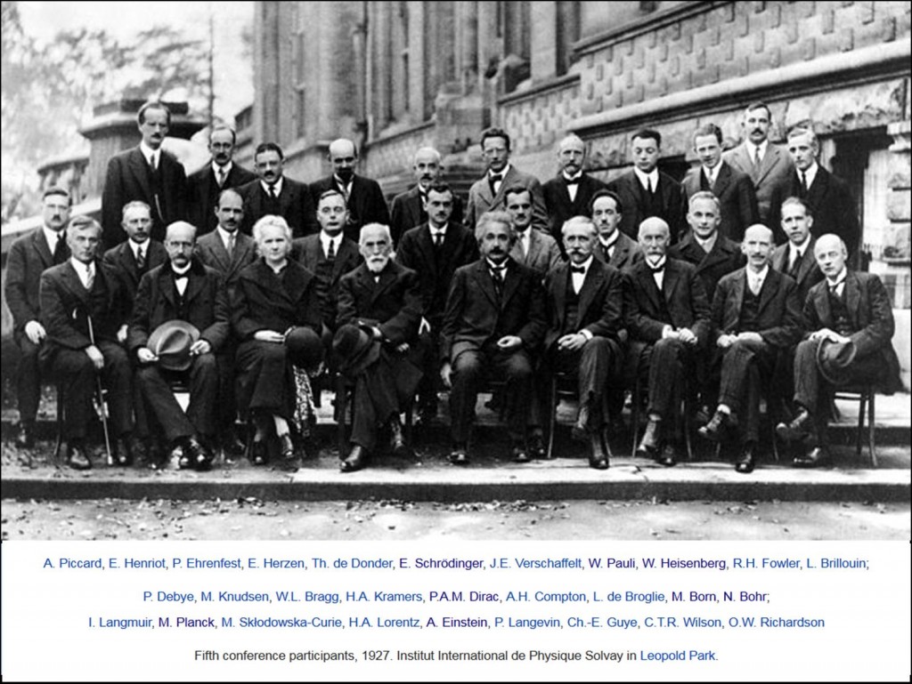
Every three years or so, Brussels hosts invitation-only meetings of the leading physicists in a current topic. These are called the Physics Solvay Conferences. The 1927 conference – “Electrons and Photons” – is still the most famous of them all, with 17 out of the 29 delegates being, or to become, Nobel Prize winners (see picture above). However, it is probably more famous for the arguments that went on outside the lecture hall than for the content of the lectures themselves. The two protagonists in these arguments were Niels Bohr and Albert Einstein. The literature covering their intense debates is extensive, running from the 1927 conference itself to the next Solvay Conference in 1930 and well beyond, and includes many different points of contention between the two giants.
Although formal notes were made of the discussions that followed the invited presentations during the 1927 conference, the meat of the Bohr-Einstein debates was continued outside of these sessions, and our only written recollections were produced, mainly from Bohr himself, often many years after the conference.
If it is possible to summarize Einstein’s chief concern in 1927, it was that he considered that quantum mechanics, even if correct insofar as it went, could not be the whole story. For instance, argued Einstein, although Heisenberg had used his matrix mechanics to show that there is a limit to how precisely we can know two properties of an object at the same time, such as position and momentum in his famous “Uncertainty Principle”, that had to be a limitation of the theory – after all, if you know exactly where a photon or an electron is, it must surely still possess an exact momentum even if, according to Heisenberg, we can only estimate it.
To get to the root of Einstein’s unhappiness with quantum mechanics, we need to go back to 1905. This is Einstein’s Wunderjahr – his miracle year – in which he wrote four radical papers that changed the way we see the world. In one of these papers, he proposed that the energy of radiation is delivered in light quanta, picturing each quantum of light behaving quite independently of its neighbours. This is perfectly normal in the world we are used to.
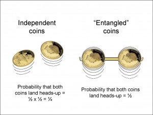
Suppose you have two coins, one in each hand, and you spin each of them up in the air at the same time. The chance that the left-hand coin will land heads-up is ½. Equally, the chance that the right-hand coin will land heads-up is also ½. So the chance that both coins will land heads-up is ½ x ½ = ¼. This is such a familiar story that it may not occur to us that this can only happen if the behaviour of each coin is independent of the other. Now, imagine instead that the behaviour of the two coins is completely interdependent – for instance, suppose that, when the left-hand coin produces heads-up then the right-hand coin also produces heads-up (and vice versa) so that they are, in a sense, “entangled”. In that case, the chance of getting two heads is ½, because there can be only two possible outcomes: both heads or both tails (see Figure 1).
Using this idea of quanta acting independently, Einstein used standard physics (Boltzmann statistics) to show that the brightness of the light emitted by a hot body agreed with measurements – at least at high frequencies. At low frequencies of radiation, though, the formula didn’t work – just as he knew it wouldn’t, because Planck had found the same thing five years earlier.
The implication was clear to Einstein: if you assume that light quanta behave independently at all frequencies, you get the wrong answer for the brightness at low frequencies, and so light quanta are clearly not behaving totally independently. He developed this idea further in two papers in 1909 in which he showed that there seem to be two aspects to light quanta – one in which quanta behave independently, like the coins, and the other, at low frequencies of light (technically, infrared radiation, which you can’t see), in which individual quanta do not seem to be acting independently, but, instead, appear to be more like waves.
What troubled Einstein was that the characteristic interdependence seemed to require instantaneous communication. Some years later, Schrödinger called this interdependence entanglement (Verschränkung). The Copenhagen school, led by Bohr, seemed to accept entanglement with equanimity. (Many years later, Einstein scathingly referred to this instantaneous connection between different parts of an entangled system as “spooky action at a distance” (spukhafte Fernwirkung) in a letter to Max Born in 1947.) However, Einstein believed that entanglement showed that the existing theory of quantum mechanics was incomplete – there had to be some deeper description of reality mediated by what was later called hidden variables. In the next page I shall tell you about the experiment that ruled out hidden variables, and the deep insight behind this experiment, as explained by John Stewart Bell in his famous paper of 1964.
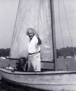
In 1933, the Nazis having stolen Einstein’s cottage and his sailing boat (which had been given to him by friends for his 50th birthday), burned his books, and put him on a list of assassination targets, he and Elsa, his wife, moved to the United States where he took up a position at the Institute for Advanced Study in Princeton, New Jersey. Two years later, he published the first paper on the paradox of entanglement with two other physicists from the Institute, Boris Podolsky and Nathan Rosen, and these three authors together became known universally as “EPR”.
Frustratingly for Einstein, the paper didn’t turn out as he had hoped. He had given it to Podolsky to write for language reasons, but the main point was “buried by the erudition”, as Einstein put it. Essentially, Einstein had wanted to formalise the ideas that he had failed to get across at the Solvay Conferences. Imagine a pair of spinning particles as suggested in Bell’s 1964 paper. Since this is a thought experiment, we shall not worry about the practical difficulties of setting up the apparatus. Assume that we have a source that emits a pair of electrons traveling in opposite directions. Before the electrons part, they are allowed to interact with each other so that they form an entangled pair. Quantum theory treats the pair as a single system, and the simplest system that is used to demonstrate the entanglement experiment is called a singlet state, in which there is no overall magnetic moment. I shall say a bit more about the singlet state below.
Two electrons in a single, entangled state
As we saw in the Quantum Spin-Filter page, there can be only two results when you measure the spin of an electron: spin-up or spin-down (in the direction that we choose to make the measurement). We sometimes use the term “wave function” for these states. We could label the states “up” and “down” or simply u and d. You can think of the wave function as representing the different possible outcomes (u and d) of a measurement on an electron before a measurement is actually made. These possible outcomes are sometimes known in quantum mechanics as basis states or, equally, basis vectors, because of their role as the basic building blocks of other states.
Now a feature of quantum mechanics is that, if you allow two electrons to interact (or, indeed, any two systems – not just electrons), then the two electrons (or systems) can be thought of as being in one of several possible combined quantum states. Furthermore, the rules of quantum mechanics say that such combined states will be formed from basis states that are, in turn, generated from the basis states of the individual electron states.
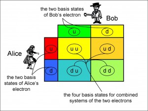
Suppose that Alice and Bob each have an electron. Figure 2 shows how the basis states of Alice’s and Bob’s electrons amalgamate to generate the basis states of the possible combined states of their two electrons.
Now, although the combined states can use all four basis vectors, imagine a combination that uses only two of them: ud and du (the first letter in each pair always refers to Alice’s electron and the second always refers to Bob’s). In such a combined state, we see from the first pair of letters, ud, that, if Alice measures her electron to be in a spin-up state then, if Bob aligns his spin-filter in the same orientation as Alice’s, he will find his electron to be in a spin-down state. From the second pair of letters, we see that, if Alice measures spin-down, then Bob measures spin-up. This will happen no matter what inclination angle Alice chooses for her spin-filter: as long as Bob chooses the same angle, then the spins of the two electrons will be orientated at the angle of the spin-filter, but in opposite directions.
For example, suppose that Alice chooses to incline her spin-filter in a horizontal direction and calls one of the two possible horizontal directions “up” and the other “down”. Then, if the result of her measurement is spin-down (so that the electron emerges from the spin-filter with a horizontally inclined spin, orientated in the direction she called “down”), then, so long as Bob measures with his spin-filter in the same horizontal direction (and not sky-ground, for instance), his result can only be spin-up.
In summary, for this particular combined state, if Alice and Bob incline their spin-filters at the same angle, then the spins they measure will always cancel out. We call this state an entangled state.
(Not every state in a combined system is an entangled state. In fact, if you configure all four of the basis vectors in the right way, you can generate states with two electrons that are quite unconnected with each other, where measuring the spin of one of the electrons tells you nothing about the outcome of measuring the spin of the other one. However, we shall only consider entangled states here.)
In fact, there are two different ways of combining the two basis states ud and du in quantum mechanics, and the two combined states that result are called (1) the singlet state and (2) one of three triplet states (the other two triplet states use the other two basis states instead). We shall concentrate on the singlet state because this is the one that arises most naturally. Imagine that the two electrons are like bar magnets. If you let the magnets interact, that is, if you bring them together, they will flip round so that the north end of each magnet sticks to the south end of the other magnet. This is the lowest-energy arrangement, and in the case of particles such as electrons, we call this arrangement the singlet state.
(When I discussed the Stern-Gerlach experiment in the Quantum Spin-Filter page, I said that, classically, the magnetic field wouldn’t change the orientation of the electron spin, and that the electron would merely precess instead. You might wonder then how the electron can flip quantum-mechanically, and why it doesn’t do so while it is traveling through the Stern-Gerlach apparatus. In fact, the electron can lose energy by releasing a photon, but the time-of-flight through the Stern-Gerlach apparatus is short enough that very few such inversions occur.)
Stretching an entangled state across the Solar System
So, if the electrons interact for long enough, they will end up in the entangled, singlet state. Suppose Alice measures the spin of one of these two electrons and Bob measures the spin of the other. In that entangled state, the electron-spin orientation that Bob finds will have the opposite orientation from that found by Alice for her electron, provided that they both choose the same inclination for their spin-filters. The astounding thing is that this applies to the measurements even if the electrons are moved apart by millions of miles – or light years – provided that the singlet state is not disturbed by another interaction during the journey.
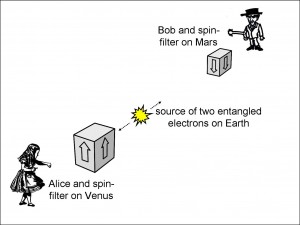
So, just to hammer the point home, suppose that the planets Venus, Earth and Mars are aligned along a radius outwards from the Sun and that Alice is on Venus, Bob is on Mars and that two entangled electrons are sent from Earth, one towards Alice and one towards Bob (Figure 3). In addition, both Alice and Bob each have a spin-filter whose alignment they can control as they wish. Notice that, since Earth is closer to Venus than Mars when they are aligned along a radius, Alice’s electron is going to reach her before Bob’s will reach him (the electrons are travelling at the same speed in opposite directions).
Let us concentrate first on what Alice sees. If she inclines her spin-filter vertically, she will find that, on average, her results will be spin-up in 50% of her measurements. This is what we expect from Figure 8 in the Quantum Spin-Filter page, which makes the point that the results of half of the measurements in any direction will be spin-up if the electron had not already interacted with something on the journey.
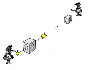
Because the two electrons comprise one entangled quantum state, Alice is able to predict with 100% certainty the outcome of every measurement that Bob makes, assuming that he aligns his spin-filter in the same vertical direction as Alice’s. If Alice detects spin-up on one measurement (Figure 4), then Bob will detect spin-down on the electron that was paired with Alice’s. If Alice turns her spin-filter the other way up and happens to detect spin-down, then she knows that Bob will detect spin-up. If she keeps her spin-filter in the spin-down orientation and does not detect an electron, then she concludes that her electron must have been spin-up, in which case, Bob will detect spin-down in his corresponding electron.
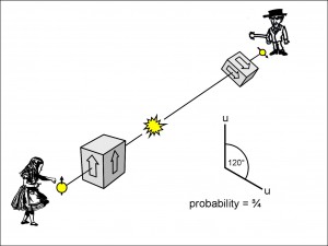
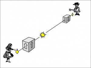
Figure 5 shows Bob measuring spin-down when his half of the electron pair finally reaches him on Mars after Alice measured spin-up on Venus. To appreciate just how surprising this is, remember that, before it reaches Alice, her electron has no spin in any given direction. The direction of the spin is chosen by Alice herself when she selects, say, a vertical alignment for her spin-filter. Once she has done this, since the entangled state has a zero net spin in any given measurement direction, she knows that Bob will definitely measure the opposite orientation if he chooses to measure in the vertical direction also.
So it seems as though Bob’s electron somehow “knows” instantaneously that it has to align itself in the same direction as the one which Alice has just chosen and to orientate itself in the opposite sense to that which Alice has just found as a result of her measurement. This apparent instantaneous “knowledge” was Einstein’s “spooky action at a distance”.
What happens if Alice and Bob are not restricted to measuring electron spin at the same alignment? That is, they don’t both have to set their spin-filters vertically, or horizontally, for instance. For illustration, we shall allow them each to choose, separately, one of three alignments for their spin-filters: 0º, 120º or 240º, where we define 0º to be in the vertical direction with the spin-filter in the “up” orientation, 120º to be in the 120º direction with the spin-filter again in the “up” direction and similarly for 240°.
First, let us look at experiments where Alice chooses 0º for her spin-filter and Bob chooses 120º (Figure 6). We assume that these choices are made at the last moment before the electrons reach Alice and Bob respectively.
After many measurements, Alice and Bob will each find that half of their measurements result in a spin-up orientation and that half result in a spin-down orientation. However, when they later compare the results of each pair of measurements and count the number of these experiments in which Alice’s results are spin-up, they find that Bob’s results are also spin-up in three-quarters of these particular experiments. By the same token, they find that, when Alice has measured spin-down, Bob has also measured spin-down in three-quarters of these particular experiments.
Now, if you just take just a casual glance at Figure 14(b) in the Quantum Spin-Fliter page, you might think I’ve made a mistake. In that figure, the probability of an electron with a vertically inclined spin-up orientation passing through a filter at 120º is given as only ¼. However, in Figure 6, with an angle of 120º between the spin-filters, I have put ¾ for the probability of both electrons being detected with a spin-up orientation.
The difference is that, in the latter figure, since Alice is shown detecting her electron with a spin-up orientation, Bob’s electron can be thought of as entering his spin-filter in a spin-down orientation, corresponding, in fact, to Figure 15(b) in the Quantum Spin-Filter page, with its associated probability of ¾. You’ll see shortly that, while this is the Copenhagen interpretation of the entanglement experiment, that interpretation must be wrong! Nevertheless, when you use the Copenhagen interpretation to calculate probabilities, it is always successful in predicting the correct values, and so I have used it here.
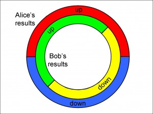
The connection between Alice’s and Bob’s results when the spin-filters are aligned at 120º to each other is illustrated in Figure 7. The outer annulus shows Alice’s results, half of which are spin-up and half of which are spin-down. The inner annulus shows Bob’s results, again split 50:50. However, I have shown the split in Bob’s results at an angle so that ¾ of his spin-up results are next to Alice’s spin-up results. The same is true for the spin-down orientation. There is no other significance to the diagram: it does not explain the ¾ split – it is included simply to show how Alice and Bob can each individually get a 50:50 split in their orientation measurements while at the same time find a match between them (both spin-up or both spin-down) for ¾ of the measurements.
In the next page, I shall tell you how Einstein thought that entanglement could be explained using hidden variables, contrary to the ideas of Bohr and his Copenhagen followers, and how John Stewart Bell finally came up with a brilliant idea that would show, once and for all, who was right.
Click here to go to the [7] Hidden Variables page