
HIDDEN VARIABLES

In the previous page on Quantum Entanglement, we saw that, if Alice on Venus and Bob on Mars both select the same angle of inclination for their spin-filters, then, no matter what angle they choose, the spins that they separately measure will always be opposites.
You might think that the electrons leaving Earth somehow “know” the alignments of both Alice’s and Bob’s spin-filters and that this knowledge can influence the results by some mechanism. However, both Alice and Bob choose the alignment of their spin-filters at the last moment before the electron reaches them, so that there is no time for Earth to know what angle the two experimenters have chosen. Neither is there time for Alice and Bob to swap this information before the measurements are over.
Nevertheless, you may be somewhat underwhelmed by all this. Isn’t the explanation obvious, even prosaic? Take the case where Alice and Bob both align their spin-filters vertically. Surely all that happens is that the two electrons are released with opposite spins from the very start? This will guarantee that Alice and Bob always measure spins with the opposite orientations. All that is necessary is for each pair of electrons to be released with the common axis of their spins aligned in a random direction so that both Alice and Bob each find a spin-up orientation as often as a spin-down orientation.
Of course, such an explanation is precisely what Einstein had in mind when he expressed his unease about quantum mechanics. He was convinced by the above explanation, that the two electrons must have hidden variables of spin in opposite directions even before any measurement is made – hidden, because quantum mechanics denies the existence of such variables before a measurement is made. This, according to Einstein, was why quantum mechanics was “incomplete”.
Despite Bohr’s enthusiastic crowd of followers who insisted on the completeness of quantum mechanics, many thought that Einstein had to be right about the electrons having hidden properties before measurement.
If the only experiment that Alice and Bob could conduct was the measurement with both spin-filters in the same vertical direction, then it would be impossible to decide between the two viewpoints. Indeed, for nearly thirty years after Einstein, Podolsky and Rosen published their paper (see discussion in the Quantum Entanglement page), the question just lay hanging there. Then, in 1964, an Irishman, John Stewart Bell, published a paper which, in the words of one (perhaps slightly too excited) physicist, was “the most profound discovery of science”. (This was Henry Stapp, a physicist at Lawrence Berkeley National Laboratory in California, who wrote it in Nuovo Cimento 29B (2) page 270 (1975).)
What Bell showed was that, in general, you can construct experiments that will have different outcomes depending upon whether quantum mechanics is complete or whether there are hidden variables underlying our understanding of quantum reality. (I should point out that I am referring here to local hidden variables. I’ll tell you what I mean by this in a moment.) Although I poked gentle fun at the enthusiasm with which his paper was received by some, this is, indeed, a profound discovery. In order to give you a flavour of what Bell was saying, let us try out his theory on the experiments where Alice and Bob are each allowed to choose, independently and at the last moment before their electron reaches them, one of three angles at which to incline their spin-filters: 0º, 120º or 240º.
After a long series of such measurements, Alice and Bob compare notes (by sending text messages between Venus and Mars). They decide to ask the question: how often are Alice’s results (that is, spin-up or spin-down) in agreement with Bob’s? In other words, how often will Alice and Bob find that they both recorded either spin-up for the same experiment or spin-down for the same experiment?
Well, we know what happens when Alice sets her spin-filter at 0º and Bob sets his at 120º. We saw in Figure 6 of the Quantum Entanglement page that, if Alice detects spin-up, then Bob will also detect spin-up in ¾ of such measurements. Correspondingly, if Alice detects spin-down, then Bob will also detect spin-down in ¾ of such measurements. This is just another way of saying that, if Alice aligns her spin-filter vertically, and Bob aligns his at 120º, then they agree on their results ¾ of the time.
Simply from the symmetry of the situation, if Alice keeps her spin-filter vertically aligned but Bob sets his spin-filter to 240º, then, again, they will find that their results agree ¾ of the time.
Of course, there is nothing special about the direction 0º that Alice chose for her spin-filter. The outcome will be exactly the same if she had chosen 120º and Bob had chosen 240º – again, ¾ of their results will agree.
Indeed, as long as the alignments of Alice’s and Bob’s spin-filters differ by 120º, their results are going to agree in ¾ of their experiments.
The only exception to this finding is when both Alice and Bob happen to choose the same angle for their spin-filter alignment. In that case, as we already know, Alice and Bob must always find that their spins are in opposite orientations. So, when both Alice and Bob choose the same angle for their spin-filter inclination, the results will never agree (they will be opposed).
So we can sum up the quantum position for the following experiment: if Alice and Bob each align their spin-filters randomly and separately in one of three directions, 0º, 120º and 240º, then, if we don’t include results where both Alice and Bob have selected the same alignment angle, their results will agree for ¾ of the time.
What we need to know now is: if we carry out the same series of experiments, with Alice and Bob setting their spin-filters randomly and independently at 0º, 120º and 240º, can the results be explained by the two electrons having predetermined properties – hidden variables – arranged in such a way that they find matching results in ¾ of the experiments (if, again, we don’t include the results where the same alignment angle is selected by both of them)?
Before we attempt to answer this question, notice we are assuming here that, when we talk of hidden variables in this sense, we assume that experiments with hidden variables will be local. By “local”, I mean that the act of measuring an electron’s spin that is determined by its hidden variables can in no way affect the outcome of the measurement of its partner’s spin. The thought experiment that I am about to describe requires Alice and Bob to choose and set the alignment of their spin filters at the last moment before each of their electrons is detected. That way, “news” of the first result cannot be transmitted instantaneously – faster than the speed of light – to the second electron. So, provided you do not believe that the universe is non-local, then the following experiment will tell you whether local hidden variables can account for the observed correlation between Alice’s and Bob’s results.
Now let us see if a local hidden-variable theory can give us the required matching in ¾ of the experiments. We already know that one of the properties that the two entangled electrons must have is that when the spin orientation of one of them, say Alice’s, is measured in any one of the three spin-filter directions, then, if Bob measures his electron using the same spin-filter direction as Alice, he will find the opposite spin orientation. As we have seen, this is what experiments show (and which is attributed to entanglement in the quantum picture).
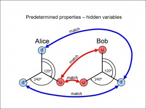
Figure 1 shows one of several possibilities for the results of measurements on electrons that have such predetermined properties – hidden variables – of spin-up and spin-down. In this example, if Alice aligns her spin-filter at 0º to measure an electron, she will find a spin-down orientation (d, according to the picture), and Bob must find spin-up when he aligns his own spin-filter at the same angle. (Although, since Alice and Bob are only looking at outcomes for electron pairs where they have each measured their own electron at different inclinations of their spin-filters, we can’t include this particular result in the final total.)
Notice that, of course, for each electron there are only two possible outcomes from a measurement at any of the three alignments: spin-up (u) or spin-down (d). Since there are only two outcomes for three alignments, there is always going to be an odd-one-out, unless all three outcomes are happen to be the same (either spin-up or spin-down at each of Alice’s three angles and vice-versa for Bob), which we shall look at shortly.
In Figure 1, the outcome which is the odd-one-out is at 120º for Alice because the outcomes at the other two alignments (at 0º and 240º) both differ from the outcome at 120º. (In other words, the odd-one-out of d, u and d is u, at 120º.) Similarly, because Bob’s outcomes have to be the opposite of Alice’s, the outcome that is the odd-one-out for Bob must also be at 120º. For a setting of 120º for Alice’s spin-filter, the experiment allows two choices of alignment for Bob’s spin-filter: 0º and 240º (because we don’t allow the same alignment as Alice’s, in accordance with the terms of the experiment). The outcomes at either of these two alignments of Bob’s will produce a match with Alice’s outcome at 120º. These two matches are shown joined by the two red connecting arrows in Figure 1.
If Alice selects one of the two remaining alignments for her spin-filter, say 240º, then there are again two possible alignments that Bob can choose for his spin-filter (again, leaving out the same alignment as Alice’s). In this case, he will find a match with Alice’s measurement at one of the angles and not the other. The match at Alice’s spin-filter alignment of 240º is shown connected by the lower of the two blue connecting arrows in Figure 1.
At Alice’s remaining alignment (at 0º), there is again, out of the two possible alignments that Bob can choose, one that matches his measurement. This match is shown by the upper of the two blue connecting arrows in Figure 1.
So, of the six different measurements that can be made between Alice and Bob when they exclude measurements with their spin-filters inclined at the same angle, there will be matching outcomes in four of them. (Just to be clear, the orientations for the spin-filters at the six different measurements are: (1) Alice 0º, Bob 120º; (2) Alice 0º, Bob 240º; (3) Alice 120º, Bob 0º; (4) Alice 120º, Bob 240º; (5) Alice 240º, Bob 0º; and (6) Alice 240º, Bob 120º.)
Of course, Alice’s electron could have hidden variables arranged in a different pattern from the one shown in Figure 1. However, excluding the cases where all outcomes are the same for the three spin-filter alignments (which we shall consider shortly), there is always going to be an odd-one-out among the three outcomes in any particular arrangement. This means that we can use the same reasoning as for Figure 1, and we shall find that there are always going to be four matches in the six different measurements that can be made between Bob and Alice.
Notice that this means that, in the first entanglement measurement, the two electrons may have the pattern of hidden variables shown in Figure 1, and in the next it may well be different. Nevertheless, the same reasoning applies to every possible pattern of hidden variables that each electron pair can have (always excepting the case where are all three outcomes are the same in a given electron).
Since Alice and Bob set their spin-filters randomly and independently at 0º, 120º and 240º, they will find that they make an equal number of measurements, on average, at each of the angles. So, for instance, if they make, say, 1,000 measurements where Alice sets her spin-filter to 0º and Bob sets his to 120º, 1,000 measurements where Alice sets her spin-filter to 0º and Bob sets his to 240º, and so on, then they will find that 4,000 out of the 6,000 possible measurements are matches.
In other words, where there are hidden variables, ⅔ of the outcomes will be matches, regardless of the pattern, provided that it conforms to the rule of Alice’s pattern and Bob’s pattern having opposite orientations (and excluding the cases where all outcomes are the same for the three spin-filter directions).
If, finally, we now include those cases where all outcomes are the same for the three spin-filter directions, what does that do to the probability of ⅔ that we have just worked out? In that case, if the hidden variables in Alice’s electron give outcomes of, say, spin-up in each of the three directions, those of Bob’s electron must each give spin-down. Hence there can be no match, regardless of the alignment of Alice’s and Bob’s spin-filters. The same will be true if the hidden variables in Alice’s electron are all spin-down and all spin-up in Bob’s electron.
So, considering every possible pattern of hidden variables that the entangled electrons can have, the probability of finding matches in the spin measurements is either ⅔ or (if there are arrangements of hidden variables where the outcomes of spin in each of the three directions are all the same for a given electron) the probability will be less than ⅔ (because there are no matches in the latter arrangement).
So we have now considered all possible permutations of hidden variables for Alice’s and Bob’s electron and we see that no more than ⅔ of the outcomes will be matches.
However, quantum mechanics predicts that ¾ of the outcomes will be matches, which is greater than the maximum possible hidden-variable matching of ⅔. So there is no arrangement of hidden variables that can mimic the results correctly predicted by quantum theory!
This doesn’t mean that the quantum-mechanical picture is necessarily correct, but it does mean that, if real experiments are designed carefully enough, it will be possible to distinguish between quantum theory and the theory with hidden variables. We need to see whether we get more than ⅔ for the fraction of results that are matches when we do the experiment (in fact, we should get ¾, according to quantum mechanics).
In order to make things clearer, the above experiment is a much simplified version of Bell’s original paper, but the flavour is the same. In fact, once Bell had devised a test to show that you can distinguish between the quantum-mechanics model and the hidden-variables model, many other workers suggested variations of Bell’s proposal, some of them similar to the above experiment, although generally involving photons instead of electrons and accordingly substituting polarisation for spin orientation. Anyway, the first experiment to test Bell’s theorem – also called Bell’s inequality to reflect the inequality of results predicted by the two models – was carried out in 1972 and from that time to the present day, all such experiments have shown agreement with quantum mechanics rather than with (local) hidden variables.
There are still some die-hards who look for loopholes in the experiments, the most important of these being (1) that the detectors are never totally efficient and so miss some of the photons and (2) that, in some cases, the time between Alice’s measurement and Bob’s measurement is long enough for a signal to be transmitted from Alice after she makes her measurement and received by Bob before he makes his measurement. The issue is not that Alice will deliberately forewarn Bob what his result should be, but that nature may somehow be connecting the two measurements to produce the fraction of matches predicted by quantum theory. However unlikely this may seem, remember that we are dealing with an unlikely phenomenon – spooky action at a distance – and so, having ruled out the more obvious explanations involving local hidden variables, we need to rule out the improbable ones too.
Such communication from Alice’s apparatus to Bob’s apparatus after Alice has made her measurement and Bob hasn’t yet made his is, as we have discussed, a local effect. In order to test quantum predictions to the hilt, Bell suggested that Alice and Bob should set the alignment of their spin-filters only after the two electrons had already left the source and were in flight. This followed a proposal by David Bohm and Yakir Aharonov, two key proponents of the hidden-variables approach.
These concerns, and, indeed, all of the other “loopholes” identified by physicists have by now been checked both individually and together by suitable experiments. The loopholes were finally plugged in 2015 in an experiment at the Kavli Institute of Nanoscience in the Netherlands, followed by the coup de grace delivered separately by teams in Vienna and in the US National Institute of Standards and Technology. This ought to extinguish, once and for all, any glowing embers that remained in the hearts of those who believed in hidden variables.
Click here to go to [8] the Wave Function Collapse page