
SELF-AWARENESS IN A TOY UNIVERSE
If the idea of multiple universes is new to you, it will almost certainly disturb you. In The Finite Multiverse, I said that “the number of parallel universes in the multiverse is unimaginably great…”. How can this be? How can they all exist? For a start, what about the conservation of energy – isn’t that violated on an unimaginable scale?
The glib answer to the last question is that within each parallel universe, energy is conserved, but, since the universes are completely independent, there can be no flow of energy between them, and so there is no need for an energy conservation law that applies to the total multiverse.

The more fundamental answer to the question of the very existence of parallel universes is that when we speak of existence, we are implicitly imagining the kind of existence that applies within our universe. We should probably have a different definition for existence outside of our own block universe. (Notice that I said “block universe” here, because, as I pointed out in The Finite Multiverse, objects – including observers – certainly exist beyond our observable universe, while these observers are nevertheless still part of our block universe.)
I shall come back to this aspect later in this page, but first I want to make the case for everything – the universe and all its constituents, the multiverse, and everything beyond – being simply a vast mathematical structure. Imagine, for a moment, that you were given the final answer to the existence of our universe: the Theory of Everything. In what language would that answer be cast? It cannot, for instance, describe quarks in terms of other particles or bundles of energy, because then we’d want to know about these new particles or what the source of the energy could be. So our answer would not be the final answer.
The clue is in the way that physics itself has to approach successively more fundamental questions about elementary particles – as you drill down, papers become increasingly more mathematical and correspondingly less descriptive. Typical of this work is the field of so-called string theory. The mathematics of string theory is so complex and exacting that it lies truly within the purview of just a small number of physicists who dedicate themselves to their field and publish the occasional review paper pre-digested for the rest of us so that we may understand it better.
Such work is strongly suggestive that the ToE will turn out to be written in the language of pure mathematics. I don’t mean that it will be a list of equations, because then you would need a cultural context in which to understand these equations. That cultural context would derive from our own universe, and the difficulty is that the universe cannot completely explain itself purely in terms of the very universe that it is trying to explain. Instead, I mean that the relations themselves would be the universe!
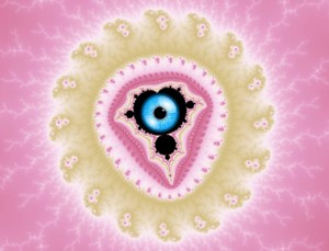
If the universe – and the multiverse – were pure mathematics, we should be less squeamish over a plethora of universes. We should regard it as we do the Mandelbrot set: an emergence of great complexity from a very simple mathematical relation (see Figure 1 for a snapshot of a part of the Mandelbrot set).
Implicit in what I have just said is that mathematics, that is, mathematical relations, exist independently of our universe. In the next section, I am going to describe a toy universe in an attempt to show you not only how that might arise, but also how mathematical constructs within such a universe might apparently be sentient and self-aware.
Building a toy universe
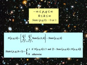
I am going to try to answer that question with a toy universe constructed entirely from the mathematical statements in Figure 2. You aren’t supposed to follow the logic of the figure because I’m going to show you equivalent representations that will be easier to follow in a moment. All you need to see just now is that there are triplets of whole numbers (integers) that I have labelled “p,q,h”, and that there is another quantity, which I have called a “State”, and which has a value of either 1 or 0 for every possible combination of p, q and h.
The mathematical statements in Figure 2 are written using the mathematical shorthand that has been developed by the human race over centuries. However, these statements are built with elements that can be considered fundamental. For instance, the numbers that are represented by p, q and h are integers, the positive ones being defined by an operation which is labelled Λ in Figure 3.
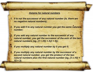
Other processes that are explicit or implicit in Figure 2 can similarly be captured in a very basic set of truths, called axioms. Figure 4 lists the five axioms that are sufficient to define arithmetic.
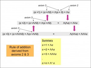
While it might seem that addition and multiplication are used in Axioms 2-5 without defining them, in fact, they are defined by these very axioms. For instance, to see how axioms 2 and 3 define addition, look at Figure 5. So that I won’t get distracted down this particular alley, I just leave Figure 5 without explanation. It has no effect on what I really want to say in this page.
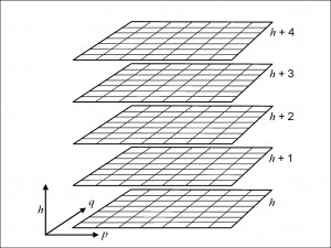
Returning to the toy universe in Figure 2, you will find it easier to see what’s going on if we plot the numbers pictorially. We can choose to handle them in any way we like, but the most revealing way will be to make a series of matrices out of the pairs of numbers p, q and to stack these matrices in a block in order of increasing values of h, as in Figure 6.
In this figure, only a sample of each matrix is shown, with each containing seven squares in the p direction and seven in the q direction, making 49 in all. They could, though, be greatly extended in all directions (although not infinitely far – it is specified in the yellow box in Figure 2 that p and q are not infinite). The quantity h is any natural number (although not infinite), as is specified in the yellow box in Figure 2.
We can now use the framework in Figure 6 to organize the statements in Figure 2 that will carry more meaning for us human beings who are used to geometric pictures (see Figure 7).
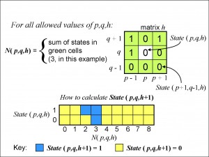
The upper part of the figure shows a sample of nine squares from one of the matrices, labelled h. The central square in the sample is labelled (p,q,h). The quantity N(p,q,h), which is shown as 3 in this example, is simply the sum of the States in the squares surrounding (but not including) the square located at p,q,h. This is the value calculated for N in the line at the top of the blue box in Figure 2.
The bottom part of Figure 7 shows how to find State (p,q,h+1), which is calculated in the bottom part of the blue box in Figure 2. In this example, as you can see from the white square surrounded by the green squares in the matrix at the top of Figure 7, the value of State (p,q,h) is 0. So we select the bottom row of the yellow-and-blue matrix in Figure 7, corresponding to State (p,q,h) = 0, and look at the square corresponding to N(p,q,h) = 3, and we find that that square is coloured blue, representing, from the Key, a value of 1 for State (p,q,h+1).
The Game of Life
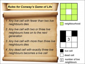
Figure 7 is equivalent to Figure 2: they say the same thing. Nevertheless, it is still not easy for us to get a feel for the spirit of the toy universe. Figure 8 displays the ideas in yet another way, using a mixture of English language and pictures. In this figure I have come clean about the provenance of the toy universe – it is actually the “Game of Life” invented by British mathematician John Conway in 1970.
I leave it to you to check that the rules in Figure 8 will give you the same result as the pictures in Figure 7 (and, if you’re feeling adventurous, that the mathematical symbols in Figure 2 do the same).
Conway thought of the squares containing a State with value 1 as a live “cell”, whereas a square that has a State with a value 0 is considered as a dead cell. The ethos behind Conway’s rules was that live cells could die either because there are too few neighbouring live cells to support them (Rule 1 in Figure 8) or because of overpopulation and consequent starvation (Rule 3). He also required exactly three neighbouring cells for reproduction (Rule 4).
The game proceeds from a starting position where all of the cells in the matrix are given individually as either dead or alive (the States for the matrix h = 0 are given as either 0 or 1, as shown in Figure 2). This would correspond to the lowest possible matrix in the block in Figure 6, setting the value of h to 0. The positions of the cells in the next matrix, where h = 1, are then calculated according to Conway’s rules in Figure 8 (or, equivalently, the picture rules in Figure 7 or, indeed, the mathematical rules of Figure 2). Once this has been done for every square in the matrix where h = 1, the distribution of cells in the subsequent matrices, where h = 2, 3, 4…, are calculated in turn.
The Game of Life owes its success, among other things, to the decade in which it was released: before 1970, the cost of computers meant that they were generally only accessible to large organisations, but, from the ’70s onwards, cheaper computers became available to many smaller businesses, and these could be programmed to play the Game of Life during quiet times. Naturally, instead of displaying the results as a block as in Figure 6, they were printed out in a sequence of large grids in the order in which each grid was calculated. When simple graphics became available on computer monitors, the output was animated by displaying the grids in chronological sequence, giving the viewer the impression of cells and structures exploding into life, imploding into the void or, occasionally, flitting across the screen as though alive.
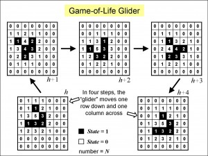
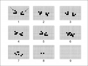
Conway’s goal had been to devise a two-dimensional world with very simple rules from which would nevertheless emerge complex and sometimes surprising structures, and in this he succeeded remarkably. In the year of the launch of the Game of Life, the “glider” was discovered by British mathematician Richard Guy. This is a five-celled structure whose shape changes in each subsequent matrix but with a period of 4 iterations. That is, in any matrix labelled, say, h, the shape of the glider will be found once again in the matrix labelled h+4. However, this repeated shape is not located in precisely the same squares of the matrix: instead, it is displaced by one row and one column – in effect, the glider has moved diagonally, taking four “ticks” to do so. Figure 9 shows the sequence for a glider travelling to the bottom right of the matrix.
In this figure, the sequence of matrices is clockwise, starting from the bottom left. Live cells are shown in black (corresponding to State = 1). The numbers in each matrix are the values of N (the number of neighbouring live cells) for any given square. You can use this picture to check your understanding of the rules. For example, using the first matrix, matrix h, and selecting the fifth row from the bottom and the second column from the left, we have a square with the number “3” in it. This is the number of neighbours with live cells around the square – one directly beneath it, one diagonally down to the right and one diagonally up to the right. Since our example square is blank – that is, it contains a dead cell, then, by Rule 4 in Figure 8, it becomes a live cell, coloured black, which you will see in the corresponding square of the next matrix, matrix h+1.
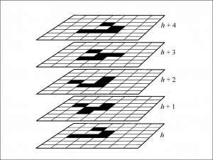
Although the glider sequence has been presented as a series of matrices in Figure 9, the mathematical structure may equally be represented using the infrastructure in Figure 6. So, in terms of a block structure, it would look like Figure 10.
In the mathematical representation of the Game of Life, in Figure 2, we use the three parameters, p, q and h, but our choice of a block of matrices to display the equation was purely a matter of expedience, as is the other option of displaying the matrices successively in order of increasing h on a computer screen, effectively making h a measure of passing time. These different ways of expressing the Game of Life are equivalent, in that the essence of the relations between the parameters is preserved: you can reconstruct one from the other. We say that these different mathematical representations are isomorphic. It is as though the statements of Figure 2 comprise the mathematical structure – the skeleton, say, of a tree: the trunk, branches and twigs – while the matrices of squares are the adornments, the leaves, which could only be displayed as you see in Figure 10 because of the structure of the underlying framework.
So the representation in Figure 10 can be thought of as a block universe. In such a picture, all moments in time are contained within the block representation – one matrix does not wait for the other to be computed first in the block universe: they are just there.
Of course, in the computer manifestation of the Game of Life, the matrices are indeed computed in sequence – how could it be otherwise? But that computer-screen representation should not be taken to mean that the root mathematical structure itself must wait to be computed for it to exist. No, the existence of the mathematical structure is completely contained in Figure 2: you only need the computer to see what it looks like.
Shortly after the glider was discovered, an American mathematician, Bill Gosper, invented a “gun” for creating them. The gun effectively has two oscillating components (see Figure 11).
When the two parts of the gun collide, they create a glider which proceeds diagonally away from the gun. The components of the gun rebound until they reach an “end stop” where they bounce back again towards each other and the cycle repeats itself. The outcome is a regular stream of gliders heading from the gun as shown.
Figure 12 shows what happens when two gliders collide (provided that they are aimed as in the illustration).
You may recognise the left-hand glider in Matrix 1 of the figure as the glider in Matrix h of Figure 9 and which travelled diagonally downwards to the right. The right-hand glider in Figure 12 is the mirror image of the left one and so it travels diagonally downwards to the left. You can check that every matrix in Figure 12 is predicted from the preceding matrix according to the Game-of-Life rules. The two gliders ultimately destroy each other, leaving no trace from Matrix 9 onwards.
Enthusiasts of the Game of Life (there are many!) have developed a range of tools to manipulate gliders including absorbing them (with an “eater”) and reflecting them directly back and at right angles without the tool destroying itself.
Gliders can be made to store and transport information. For example, they can be used like a train of electronic pulses in a computer where a value “1” is assigned to a glider and “0” is assigned to the absence of a glider (for instance, the space in a train of gliders left after one has been destroyed). In other words, the stream of gliders can represent a train of binary digits – bits – containing information.
Implementing logic in the Game of Life
Surprisingly, the glider-handling tools can be used within the Game of Life to synthesise the three basic operations of logic: AND, OR and NOT. The meanings of these three operations are illustrated in Figure 13.
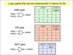
At the top is the AND gate. This compares two bits, each having a value of 0 or 1, which are fed into the gate, producing an output as a result of the comparison. The gate is portrayed by a “U” on its side, with two input lines entering it from the left and an output line leaving it to the right. The results of the comparison are listed on the accompanying table (called a truth table). Essentially, the AND gate only produces a value of 1 if both of the inputs are also 1; otherwise, it produces 0.
The symbol for the OR gate is similar to that for the AND gate except that it is pointed. However, as you can see from the truth table, the output is always 1 unless both inputs are 0.
The NOT gate is simpler because it requires only one input, and the output is just the opposite value of the input.
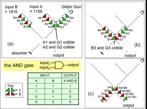
It might seem that logic gates are too sophisticated to be implemented with such simple rules as those underlying the Game of Life, and so, in Figure 14, I have drawn a scheme showing how to construct an AND gate.
Windows (a), (b) and (c) of Figure 14 are snapshots of the AND gate in order of increasing time. A glider gun fires a continuous stream of gliders diagonally down and to the left. In (a) you can see two inputs, A and B, represented by two streams of gliders moving diagonally down and to the right. In fact, as you will see from the Key, the A and B inputs each contain two blank gliders – these are spaces where you would normally expect a glider, the spaces symbolising 0. So, starting from the glider at the front of the queue and working backwards, the input A (A1, A2, A3, A4) is 1,1,0,0 and the input B (B1, B2, B3, B4) is 1,0,1,0. Pairing the first bit of the A input, 1, with the first bit of the B input, which is also 1, we should expect that the first bit of the output train, from the truth table, will also be 1. The complete output train should be 1,0,0,0 because none of the remaining three pairs of bits, namely 1,0 and 0,1 and 0,0, will produce an output of 1 according to the truth table.
Each of the two gliders at the front of the A input stream, A1 and A2 collides with each of the two gliders from the glider gun, G1 and G2, in succession. As we have seen in Figure 12, such collisions wipe out both gliders, leaving two spaces – blank gliders – in front of the stream from the gun, as you can see in (b). The first of these spaces, G1, reaches the crossroads with the B input line at the same time as the first glider from the B stream, B1. So this B1 glider sails over the crossroads unmolested, forming the first glider – corresponding to a bit of value 1 – in the output stream as shown in (c). In the figure, I have written this in symbols: A1 Λ B1 where “Λ” is the conventional symbol for the AND operation (please don’t confuse this with my use of the same symbol for the successor function in Figure 5).
The second bit of the B input stream, B2, is a space and this also passes into the output stream as the second bit, A2 Λ B2, corresponding to a value of 0.
The last two gliders from the glider gun, G3 and G4, were not destroyed by the corresponding inputs in the A stream, A3 and A4, because these were blank spaces.
The third bit of the B input, B3, is a glider, and this collides with the first of the two gliders remaining in the stream from the gun, G3, annihilating it. So there is no glider left for the third bit of the output, which is therefore 0 again.
The fourth bit of the B input, B4, is a space, so that there is no collision with the last glider from the gun, G4, and so this gun glider carries on harmlessly to be absorbed by the absorber at the end of the gun line. Meanwhile, as there is again no glider to contribute to the last bit of the output, that bit is again 0.
So, as you will see from (c), the output stream is 1,0,0,0, as we required.
OR and NOT gates can be constructed in the Game of Life using similar tricks. All logical and computational operations can be carried out using these three basic logic gates, AND, OR and NOT. (In fact, you only need two logic gates: a NOT gate together with either an AND or an OR gate to build all possible logic gates or, equivalently, to satisfy all possible truth tables. However, you can perform some operations more efficiently using all three logic gates than if you use just two.)
Running a Universal Turing Machine in the Game of Life
Remarkably, using the principles of the three basic logic gates, it is possible to design Turing Machines within the Game of Life, a feat accomplished by Paul Rendell in 2000. A Turing Machine is an imaginary apparatus for manipulating symbols on a tape according to a set of rules. It is useful as a tool for thinking about computing because, if something can be computed, it can be done using a Turing Machine. (The Turing Machine, and the history behind it, are described in Andrew Hodges’ wonderful biography of British mathematician Alan Turing.)
In a Turing Machine implemented in the Game of Life, each symbol on the tape is represented by a group of three gliders. Since each glider can be present or absent, this allows us to represent a total of 2 x 2 x 2 = 8 symbols. The tape itself is a ladder of cells with each cell containing a symbol represented by up to three gliders. The gliders are confined to the cells with an ingenious arrangement for reflecting the gliders back into the cells when they approach the “walls” of the cells. Movement of the tape through the machine is achieved by allowing the gliders to leak through temporary holes in the cell walls when required.
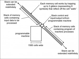
A Turing Machine can only perform the operations that it was designed to do, but there is an extension of this called the Universal Turing Machine, or UTM, which can be made to perform the operations of any Turing Machine. Therefore, a UTM can emulate any computer. A decade after his success in implementing a Turing Machine in the Game of Life, Paul Rendell devised a UTM using the same principles – see Figure 15 and this Youtube video.
In this figure, the tape is divided into two “stacks”, one going up to the top left and the other going down to the bottom right. They are diagonal, of course, because the gliders that carry the information move diagonally. The architecture at the junction of the two stacks controls the direction of information in the stacks and sends relays of gliders into and out of the programmable machine. Although the information at the start of the process is contained in a limited number of cells in either stack, data will generally have to be added to the stacks, both as part of the working of the machine and as the machine output. So it is important that the stacks can be extended without limit as necessary, in either direction as shown in the figure.
One of the stacks contains instructions for programming a Turing Machine to process data in the way we wish – for instance, to multiply numbers together or to find the largest number in a sequence. The other stack contains the numbers themselves – the input data.
The details of the construction are not important for our purposes: what matters here is the very fact that it is possible to implement a UTM in the Game of Life.
“I compute, hence I am.”
And here is why it matters: since you can implement a UTM in the Game of Life, and since a UTM can emulate any computer, it must be possible to program this Game of Life UTM with the Game of Life itself!
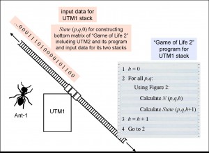
Figure 16 shows the (imaginary) screen of my computer, which I have programmed to run a Game of Life, which I shall label “Game of Life 1”. In this particular Game of Life, I have included a UTM which I have labelled UTM1. I have also included an ant, called Ant-1, which, itself, contains another UTM. So my Game of Life 1 is running two UTMs – one called UTM1 and the other is inside an ant called Ant-1.
The screen of my computer is not very high-res, but you can imagine me peering closely at the screen and just making out the individual gliders and all the other components buzzing within the stacks and within the bodies of UTM1 and Ant-1 like tiny, frenzied insects.
So what is UTM1 doing? First of all, it reads the program contained in the lower-right stack. The program that I have loaded into the stack is just the set of instructions in Figure 2, which, as we saw earlier, is the set of mathematical statements for implementing the Game of Life. We shall call this program in UTM1’s stack “Game of Life 2”. So UTM1, which is a computer running in the Game of Life is now, itself, set to implement the Game of Life!
UTM1 begins by reading the data in the upper-left stack. This data is purely a set of “1”s and “0”s representing the live and dead cells in the bottom matrix of “Game of Life 2” which UTM1 will construct. Because the Game of Life is conventionally represented on a grid, UTM1 loads and reads the data according to a convention that relates the one-dimensional series of “1”s and “0”s to the two-dimensional grid, for example, a square spiral pattern centred at p = q = 0.
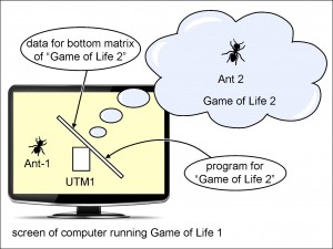
In Figure 17, you can see Ant-1 within the Game of Life 1 on my computer screen. You can also see that Game of Life 2, which is the program that Game of Life 1 is running, contains another ant, which I have called Ant-2. Of course, Ant-2 also contains a UTM!
I have drawn Game of Life 2 in a think-bubble because it is not actually displayed on the monitor screen. You can see UTM1 and Ant-1 on the monitor, and, as I said, if you peer closely, you can see that UTM1 is active, running Game of Life 2. The fact that Game of Life 2 is not displayed on a computer screen is a technicality. I could equally well not have displayed Game of Life 1 on the computer screen, but it would still be running on my computer, just as Game of Life 2 is running on UTM1.
Why have I included ants in my programs? Well, in addition to the UTM in its brain, I have programmed it with the ability to detect features of its environment – for instance, it can send out groups of gliders that can be made to bounce back and thereby convey information to the ant about its environment. (I haven’t really programmed an ant, of course – this is just a thought experiment! – but it would be possible in principle.) The UTM in the ant’s brain can use this information to build a model of the ant’s environment, which, of course, includes the UTM of the ant itself! (This model will be incomplete for reasons that Turing himself explained, and I shall tell you more about this incompleteness in the page about Gödel’s incompleteness theorems.)
So, remarkably, since Ant-1 and Ant-2 are each aware of their own construction and that they each compute, then, Descartes-style, they may be said, in a sense, to be self-aware! “I compute, hence I exist!”
Ant-1 will be aware that there is an Ant-2 embedded within the program and input data contained in UTM1’s stacks. Given a little licence, we can even imagine Ant-1 being smug about the fact that Ant-2 is not displayed on a computer screen, and so Ant-1 thinks that the existence of Ant-2 is in some sense less valid than its own, because Ant-2 is just a mathematical structure. The irony, of course, is that Ant-1 is, itself, “just” a mathematical structure – remember that the computer program running Game of Life 1 is essentially the static mathematical structure of Figure 2.
Of course, the mathematical structure of our own universe and multiverse is more complex than that of the Game of Life, but we share with Ant-1 and Ant-2 the essence of our self-awareness and the conviction that we exist.
Nothing in this chapter proves that our universe is a mathematical structure, but the Game of Life shows that a mathematical structure can be complex enough to support an object that interacts with its environment in such a way that it “sees” its world as a multi-dimensional structure containing elementary “particles” (live cells) behaving according to a set of rules. There is nothing that the object can do to prove that the particles that it observes do not actually exist – and, in fact, from the object’s perspective, these elementary particles exist just as surely as does the object itself (and they both derive from the same set of rules).
Postscript
When you watch a Universal Turing Machine running in the Game of Life (see this Youtube video) it is natural to assume implicitly that Ant is created every time the Game of Life in Figure 16 starts running. Without thinking, you presume that, before you start the program, Ant has no existence, let alone self-awareness.
But then remember that the program is isomorphic to the static mathematical structure in Figure 2. That mathematical structure is still there even when the computer isn’t running the program. For a start, it exists in the pattern of electric fields within the semiconductors that store the computer program. But that pattern was preceded by the one in the brain of the computer programmer before it was coded into the computer.
As I said above, mathematical relations exist independently of our universe. The mathematical structure in John Conway’s brain was not invented by him – he discovered it, just as Mandelbrot discovered the Mandelbrot set! Like Jack Nicholson’s caretaker, the structure has always been there! I shall return to this theme after I have described the mathematical structure of the Plexus.
Click here to go to Gödel’s Incompleteness Theorems [17]